Chapter 4 Deep Learning

• In recent years there has been a lot of hype about Deep Learning (DL)
• Deep Neural Networks are Neural Networks with many hidden layers
• Several heuristics are often used in DL:
  • Dropout. Some connections are ignored during learning: regularization
  • ReLU units: (avoid gradient vanishing)
  • Transfer learning: use weights already trained with different datasets (and maybe fine-tune training with your database)
• DL includes some novel architectures
  • Convolutional Neural Networks (CNN): images
  • Long Short Term Memory (LSTM): time series
• Improvements outside Machine Learning theory
  • Cloud environments such as Google Colab
  • Hardware: GPUs
  • Software packages: e.g. tensorflow (using keras as interface), H2O, fast.ai, torch, etc.
  • Funding: Netflix, Google, Facebook…

4.1 Regression with deep Neural Networks

This is the task in Chapter 10.9 of An Introduction to Statistical Learning. The code is from the R torch version.

1. First, data is not completely loaded into memory with a standard variable. Instead, a dataset is configured that will load data as it is needed.

library(torch)
library(luz) # high-level interface for torch
library(torchvision) # for datasets and image transformation
library(torchdatasets) # for datasets we are going to use
# library(zeallot)
# Load datasets
transform <- function(x) {
  x %>% 
    torch_tensor() %>% 
    torch_flatten() %>% 
    torch_div(255)
}
train_ds <- mnist_dataset(
  root = ".", 
  train = TRUE, 
  download = TRUE, 
  transform = transform
)

## Dataset <mnist> (~12 MB) will be downloaded and processed if not
## already available.
## Dataset <mnist> loaded with 60000 images.

test_ds <- mnist_dataset(
  root = ".", 
  train = FALSE, 
  download = TRUE,
  transform = transform
)

## Dataset <mnist> (~12 MB) will be downloaded and processed if not
## already available.
## Dataset <mnist> loaded with 10000 images.

length(train_ds)

## [1] 60000

length(test_ds)

## [1] 10000

# Show some example image
image(train_ds$data[1, 1:28, 1:28])

train_ds$targets[1] - 1

## [1] 5

2. Then, the NN is configured

modelnn <- nn_module(
  initialize = function() {
    self$linear1 <- nn_linear(in_features = 28*28, out_features = 256)
    self$linear2 <- nn_linear(in_features = 256, out_features = 128)
    self$linear3 <- nn_linear(in_features = 128, out_features = 10)
    
    self$drop1 <- nn_dropout(p = 0.4)
    self$drop2 <- nn_dropout(p = 0.3)
    
    self$activation <- nn_relu()
  },
  forward = function(x) {
    x %>% 
      
      self$linear1() %>% 
      self$activation() %>% 
      self$drop1() %>% 
      
      self$linear2() %>% 
      self$activation() %>% 
      self$drop2() %>% 
      
      self$linear3()
  }
)
print(modelnn())

## An `nn_module` containing 235,146 parameters.
## 
## ── Modules ──────────────────────────────────────────────────────
## • linear1: <nn_linear> #200,960 parameters
## • linear2: <nn_linear> #32,896 parameters
## • linear3: <nn_linear> #1,290 parameters
## • drop1: <nn_dropout> #0 parameters
## • drop2: <nn_dropout> #0 parameters
## • activation: <nn_relu> #0 parameters

# Configure optimizer
modelnn <- modelnn %>% 
  setup(
    loss = nn_cross_entropy_loss(),
    optimizer = optim_rmsprop, 
    metrics = list(luz_metric_accuracy())
  )

3. Once everything is prepared, the fitting process of the NN is really executed

system.time(
   fitted <- modelnn %>%
      fit(
        data = train_ds, 
        epochs = 1, #15, 
        valid_data = 0.2,
        dataloader_options = list(batch_size = 256),
        verbose = TRUE
      )
 )
plot(fitted)

4. Finally, accuracy can be assessed

accuracy <- function(pred, truth) {
   mean(pred == truth) }

# gets the true classes from all observations in test_ds.
truth <- sapply(seq_along(test_ds), function(x) test_ds[x][[2]])

fitted %>% 
  predict(test_ds) %>% 
  torch_argmax(dim = 2) %>%  # the predicted class is the one with higher 'logit'.
  as_array() %>% # we convert to an R object
  accuracy(truth)

4.2 Generative Networks

• Generative Models produce new data with the same underlying probability distribution of observed data
• Generative Models are Unsupervised Learning techniques
• Generative Adversarial Networks use Supervised Learning (regression and classification) to build an unsupervised generative model

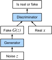
(Figure by Zhang, Aston and Lipton, Zachary C. and Li, Mu and Smola, Alexander J. - https://github.com/d2l-ai/d2l-en, CC BY-SA 4.0, https://commons.wikimedia.org/w/index.php?curid=152265649)

This code is from RGAN

library(torch)
library(RGAN)

# Sample some toy data to play with.
data <- sample_toydata()

# Transform (here standardize) the data to facilitate learning.
# First, create a new data transformer.
transformer <- data_transformer$new()

# Fit the transformer to your data.
transformer$fit(data)

# Use the fitted transformer to transform your data.
transformed_data <- transformer$transform(data)

# Have a look at the transformed data.
par(mfrow = c(3, 2))
# Margins!!
par(mar=c(1,1,1,1))
plot(
    transformed_data,
    bty = "n",
    col = viridis::viridis(2, alpha = 0.7)[1],
    pch = 19,
    xlab = "Var 1",
    ylab = "Var 2",
    main = "The Real Data",
    las = 1
)

# No cuda device!!
device <- "cpu"

# Now train the GAN and observe some intermediate results.
res <-
    gan_trainer(
        transformed_data,
        eval_dropout = TRUE,
        plot_progress = TRUE,
        plot_interval = 600,
        device = device
    )